Input space optimization
In this toy example, we directly optimize point configurations in \(\mathbb{R}^2\). The example is motivated by the toy experiments from the following paper:
Note: In all the following examples, we use the \(l_1\) norm during Vietoris-Rips persistent homology computation (whereas the paper mentioned above uses \(l_2\)).
[1]:
%load_ext autoreload
%autoreload 2
[2]:
import torch
import matplotlib.pyplot as plt
from torchph.pershom import vr_persistence_l1

device = "cuda"
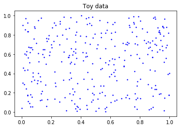
Data
The toy data generated for this example is sampled from a 2D uniform distribution in \([0,1]^2\). In particular, we sample 300 points.
[3]:
np.random.seed(1234)
toy_data = np.random.rand(300, 2)

plt.figure()
plt.plot(toy_data[:, 0], toy_data[:, 1], 'b.', markersize=3)
plt.title('Toy data');
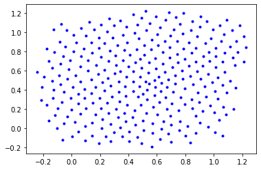
Example 1
Task: Optimize for uniform distribution of H0 lifetimes.
[6]:
X = torch.tensor(
    toy_data,
    device=device,
    requires_grad=True)

opt = torch.optim.Adam([X], lr=0.01)

for i in range(1,100+1):
    pers = vr_persistence_l1(X, 1, 0)
    h_0 = pers[0][0]

    lt = h_0[:, 1] # H0 lifetimes
    loss = (lt - 0.1).abs().sum()

    if i % 20 == 0 or i == 1:
        print('Iteration: {:3d} | Loss: {:.2f}'.format(i, loss.item()))

    opt.zero_grad()
    loss.backward()
    opt.step()

X = X.cpu().detach().numpy()
plt.figure()
plt.plot(X[:, 0], X[:, 1], 'b.');
Iteration:   1 | Loss: 15.35
Iteration:  20 | Loss: 5.85
Iteration:  40 | Loss: 3.74
Iteration:  60 | Loss: 2.66
Iteration:  80 | Loss: 2.00
Iteration: 100 | Loss: 1.69
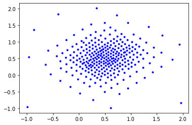
Example 2
Task: Minimize (non-essential) H0 lifetimes (i.e., a slightly modified as in Brüel-Gabrielsson et al., arXiv 2019, Fig. 1 top-right)
[7]:
X = torch.tensor(
    toy_data,
    device=device,
    requires_grad=True)

opt = torch.optim.Adam([X], lr=0.01)

for i in range(1,100+1):
    pers = vr_persistence_l1(X, 1, 0)
    h_0 = pers[0][0]

    lt = h_0[:, 1] # non-essential H0 lifetimes
    loss = lt.sum()

    if i % 20 == 0 or i == 1:
        print('Iteration: {:3d} | Loss: {:.2f}'.format(i, loss.item()))

    opt.zero_grad()
    loss.backward()
    opt.step()

X = X.cpu().detach().numpy()
plt.figure()
plt.plot(X[:, 0], X[:, 1], 'b.');
Iteration:   1 | Loss: 14.74
Iteration:  20 | Loss: 7.25
Iteration:  40 | Loss: 5.65
Iteration:  60 | Loss: 4.87
Iteration:  80 | Loss: 4.43
Iteration: 100 | Loss: 4.10
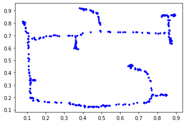
Example 3
Task: Increase (non-essential) H0 lifetimes (i.e., a slightly modified version as in Brüel-Gabrielsson et al., arXiv 2019, Fig. 1 top-left)
[8]:
X = torch.tensor(
    toy_data,
    device=device,
    requires_grad=True)

opt = torch.optim.Adam([X], lr=0.01)

for i in range(1,100+1):
    pers = vr_persistence_l1(X, 1, 0)
    h_0 = pers[0][0]

    lt = -h_0[:, 1] # non-essential H0 lifetimes
    loss = lt.sum()

    if i % 20 == 0 or i == 1:
        print('Iteration: {:3d} | Loss: {:.2f}'.format(i, loss.item()))

    opt.zero_grad()
    loss.backward()
    opt.step()

X = X.cpu().detach().numpy()
plt.figure()
plt.plot(X[:, 0], X[:, 1], 'b.');
Iteration:   1 | Loss: -14.74
Iteration:  20 | Loss: -26.88
Iteration:  40 | Loss: -33.22
Iteration:  60 | Loss: -38.43
Iteration:  80 | Loss: -43.28
Iteration: 100 | Loss: -47.87