Differentiable Vietoris-Rips persistent homology
In this example, we essentially reproduce the toy experiment from
Notation
\(S\) is a mini-batch of points \(x \in \mathbb{R}^2\) of size \(|S|=b\)
\(\dagger(S)\) is the set of death-times obtained from the VR PH of \(S\)
\(\eta\) is the desired lifetime value (in our case \(\eta=2\))
\(\varepsilon_t, t \in \dagger(S)\) are the pairwise distance values of points in \(S\)
Learning task
Given a 2D point cloud (sampled from three Gaussians), find a mapping \(f_\theta: \mathbb{R}^2 \to \mathbb{R}^2\) (implemented via a simple MLP) such that the connectivity loss
is minimized over mini-batches of samples (\(S\)).
[1]:
%load_ext autoreload
%autoreload 2
[2]:
# PyTorch imports
import torch
import torch.nn as nn
from torch.utils.data import DataLoader
from torch.utils.data.dataset import Subset, random_split, TensorDataset

# matplotlib imports
import matplotlib
import matplotlib.pyplot as plt
from matplotlib.colors import LinearSegmentedColormap

# misc
from collections import defaultdict, Counter
from itertools import combinations

# imports from torchph
from torchph.pershom import vr_persistence_l1


def apply_model(model, dataset, batch_size=100, device='cpu'):
    """
    Utility function which applies ``model`` to ``dataset``.
    """
    dl = torch.utils.data.DataLoader(
        dataset,
        batch_size=batch_size,
        num_workers=0
    )
    X, Y = [], []

    model.eval()
    model.to(device)

    with torch.no_grad():
        for x, y in dl:

            x = x.to(device)
            x = model(x)

            # If the model returns more than one tensor, e.g., encoder of an
            # autoencoder model, take the first one as output...
            if isinstance(x, (tuple, list)):
                x = x[0]

            X += x.cpu().tolist()
            Y += (y.tolist())

    return X, Y

# Run everything on the GPU
device = "cuda"
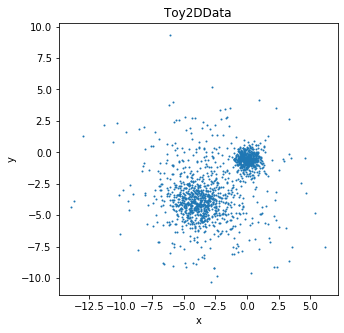
Toy data
First, we create a toy dataset with 2D points sampled from three Gaussians with different means and covariances. In particular, we create a class which derives from torch.utils.data.Dataset so we can later conveniently use PyTorch’s dataloader.
[3]:
class Toy2DData(torch.utils.data.Dataset):
    def __init__(self, n_samples_by_class):
        super().__init__()
        X = []
        Y = []
        self.mus = [
            [4.0,4.0],
            [3.0,3.0],
            [0.0,0.5]
        ]
        self.sigmas = [
            [1.0,1.0],
            [3.0,3.0],
            [0.5,0.5]
        ]

        for y, (m, s) in enumerate(zip(self.mus, self.sigmas)):
            X_class = torch.randn((n_samples_by_class, 2))* torch.tensor(s) - torch.tensor(m)
            X.append(X_class)
            Y += n_samples_by_class*[0]

        self.X = torch.cat(X, dim=0)
        self.Y = Y

    def __len__(self):
        return len(self.Y)

    def __getitem__(self, item):
        return self.X[item], self.Y[item]

    def __iter__(self):
        return zip(self.X, self.Y)
Let’s sample 1,500 points from this dataset (500 per Gaussian) and visualize the configuration in \(\mathbb{R}^2\).
[4]:
dataset = Toy2DData(500)

plt.figure(figsize=(5,5))
X = dataset.X.numpy()
plt.plot(X[:,0],
         X[:,1], '.',markersize=2);
plt.xlabel('x')
plt.ylabel('y')
plt.title('Toy2DData');
Model & Optimization
We implement our mapping \(f_\theta\) as a simple MLP with three linear layers, interleaved with LeakyReLU activations. For optimization we use ADAM. We run over 30 epochs with a learning rate of \(0.01\) and over 20 additional epochs with a learning rate of \(0.001\).
[5]:
model = nn.Sequential(
    nn.Linear(2, 10),
    nn.LeakyReLU(),
    nn.Linear(10, 10),
    nn.LeakyReLU(),
    nn.Linear(10, 2)
).to(device)


opt = torch.optim.Adam(
    model.parameters(),
    lr=0.01)

dl = DataLoader(
    dataset,
    batch_size=50,
    shuffle=True,
    drop_last=True)

# Get the transformed points at initialization
transformed_pts = [apply_model(model, dataset, device=device)[0]]

iteration_loss = []
for epoch_i in range(1, 51):
    epoch_loss = 0

    model.train()

    # Learning rate schedule
    if epoch_i == 20:
        for param_group in opt.param_groups:
            param_group['lr'] = 0.001
    if epoch_i == 40:
        for param_group in opt.param_groups:
            param_group['lr'] = 0.0001

    # Iterate over batches
    for x, _ in dl:

        x = x.to(device)

        # Compute f_\theta(S)
        x_hat = model(x)

        """
        Loss computation (for \eta=2):

        (1) Compute VR persistent homology (0-dim)
        (2) Get lifetime values
        (3) Compute connectivity loss

        Note that all barcode elements are of the form (0,\varepsilon_t)!
        """
        loss = 0
        pers = vr_persistence_l1(x_hat, 0, 0)[0][0] # VR PH computation
        pers = pers[:, 1]                           # get lifetimes
        loss = (pers - 2.0).abs().sum()             #

        # Track loss over iterations and epochs
        iteration_loss.append(loss.item())
        epoch_loss += loss.item()

        # Zero-grad, backprop, update!
        opt.zero_grad()
        loss.backward()
        opt.step()

    print('Epoch: {:2d} | Loss: {:.2f}'.format(epoch_i, epoch_loss/len(dl)), end='\r')

    x_hat, _ = apply_model(
        model,
        dataset,
        device=device)
    transformed_pts.append(x_hat)
Epoch: 50 | Loss: 37.76
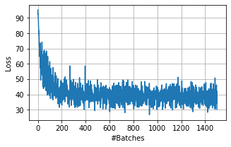
Visualize the loss over all iterations …
[6]:
plt.figure(figsize=(5,3))
plt.plot(iteration_loss)
plt.xlabel('#Batches');
plt.ylabel('Loss');
plt.grid();
Visualization
To study the effect of minimizing the connectivity loss, we freeze the model and check how the min/max/avg. lifetime changes over (1) epochs.
[7]:
def track_persistence_info(points, batch_size, N):

    ds = TensorDataset(
        torch.tensor(points),
        torch.tensor([0]*len(points)))

    dl = DataLoader(
        ds,
        batch_size=batch_size,
        shuffle=True,
        drop_last=True)

    stats = defaultdict(list)
    for i in range(N):
        for x,_ in dl:

            x =  x.to(device)

            pers = vr_persistence_l1(x, 0, 0)[0][0]
            pers = pers[:, 1]

            stats['alpha'].append(pers.min().item())
            stats['beta'].append(pers.max().item())
            stats['avgeps'].append(pers.mean().item())

    return stats
[8]:
def visualize(transformed_pts, ax):

    pts = np.array(transformed_pts)
    x, y = pts[:,0], pts[:,1]

    ax.plot(x, y, '.', **{'markersize':2, 'color':'black', 'alpha': 0.3})

    stats = track_persistence_info(
        pts,
        50,
        10)

    ax.set_title(r'$\widehat{\alpha},\widehat{\varepsilon}, \widehat{\beta}$ = ' + '{:.2f}, {:.2f}, {:.2f}'.format(
                    np.mean(np.array(stats['alpha'])),
                    np.mean(np.array(stats['avgeps'])),
                    np.mean(np.array(stats['beta']))),
                  position=(0.04,0.02),
                  fontsize=12,
                  horizontalalignment='left',
                  bbox=dict(facecolor='white', alpha=0.7));
From left to right: Initialization (epoch 0), after 5 epochs, after 50 epochs:
[9]:
fig, axes = plt.subplots(1, 3, figsize=(14, 4))
for i, epoch in enumerate([0, 5, 50]):
    ax = axes[i]
    visualize(transformed_pts[epoch], ax)
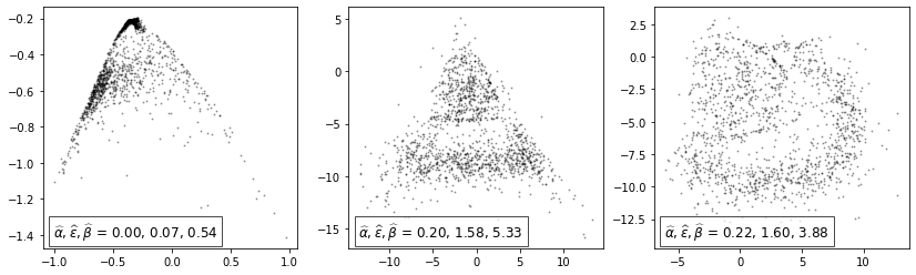
Note: Observe how the \([\hat{\alpha}, \hat{\beta}]\) interval gets tighter throughout the epochs and \(\hat{\varepsilon}\) gets closer to \(\eta=2\). However, arranging batches of size 50 in the desired manner is impossible in \(\mathbb{R}^2\) which is why the actual value of \(2\) is never reached (for details see paper).